
How to Upload (Pre)-Annotations to Roboflow
I’m a big fan of Roboflow. They have one of the most user-friendly labeling interfaces. I have been using it for quite some time now. However, only recently did I learn that you can also upload annotations and predictions programmatically. This creates some new possibilities like:
- Programmatically importing pre-existing datasets.
- Uploading pre-annotations to speed up the labeling process.
- Creating active learning loops.
- And much more.
Sadly, the documentation is not entirely clear on how to use this feature. So, in this post, I will show you how to use the Roboflow Python SDK to upload annotations and predictions to your Roboflow projects.
Preparing the Environment
Before we can start, we have to gather some information first.
You will need your Roboflow API key, the name of your workspace, and the name of your project.
The workspace and project name can be found in the project URL: https://app.roboflow.com/workspaces/<your-workspace>/projects/<your-project>.
You can find your API key at: https://app.roboflow.com/<your-workspace>/settings/api.
Let’s store these values in a .env file or in environment variables using the following names:
ROBOFLOW_API_KEYROBOFLOW_WORKSPACEROBOFLOW_PROJECT
The final step we need to take is to install the Roboflow SDK. You can do this using pip.
pip install roboflow
After that is done, we should be ready to get started.
Upload Annotations and Predictions
We will use the single_upload API endpoint to upload our annotations and predictions. To use this function, we need three files:
- The image file. Make sure this image has no orientation metadata, read here more why in my blog post: How to avoid orientation bugs in Computer Vision labeling?.
- The annotation file. This file should be in the YOLO text format for either bounding boxes (
class_idx x_center y_center width height) or polygons (class_idx x_1 y_1 ... x_n y_n), with normalized coordinates between 0 and 1. - The label mapping file. The i-th line in this file contains the name of the corresponding class.
After you have prepared all these files, you can upload them to Roboflow using the following code.
from roboflow import Roboflow
import os

rf = Roboflow(api_key=os.environ["ROBOFLOW_API_KEY"])
rf_workspace = rf.workspace(os.environ["ROBOFLOW_WORKSPACE"])
rf_project = rf_workspace.project(os.environ["ROBOFLOW_PROJECT"])

image_path = "path/to/your/image.jpg"
label_path = "path/to/your/label.txt"
label_map_path = "path/to/your/label_mapping.txt"

response = rf_project.single_upload(
    image_path=str(image_path),
    annotation_path=label_path,
    annotation_labelmap=str(label_map_path),
    batch_name="my_batch",
    is_prediction=True,
)
This code snippet can be used to upload both annotations and predictions.
The only difference is the is_prediction parameter.
If it is set to False, Roboflow directly adds the annotations to your dataset.
If this parameter is set to True, Roboflow will create a new annotation job with the name specified in the batch_name parameter.
That way, the labelers still need to review the annotations and optionally adjust them before they are added to the dataset.
If you use this function to upload multiple images with their predictions using the same batch_name, Roboflow will group them together in a single annotation job.
This way, you have full control over which images and their pre-annotations end up in which annotation job.
How does it look like in the UI?
If you specified is_prediction=False, the annotation will be present in your dataset like any other human-made annotation.
If you specified is_prediction=True, you must look for the annotation job before you can see the pre-annotations in the UI.
You can find it by clicking on ‘Annotate’ in the left menu, which will show you a new unassigned annotation job with the name you specified in the batch_name parameter.
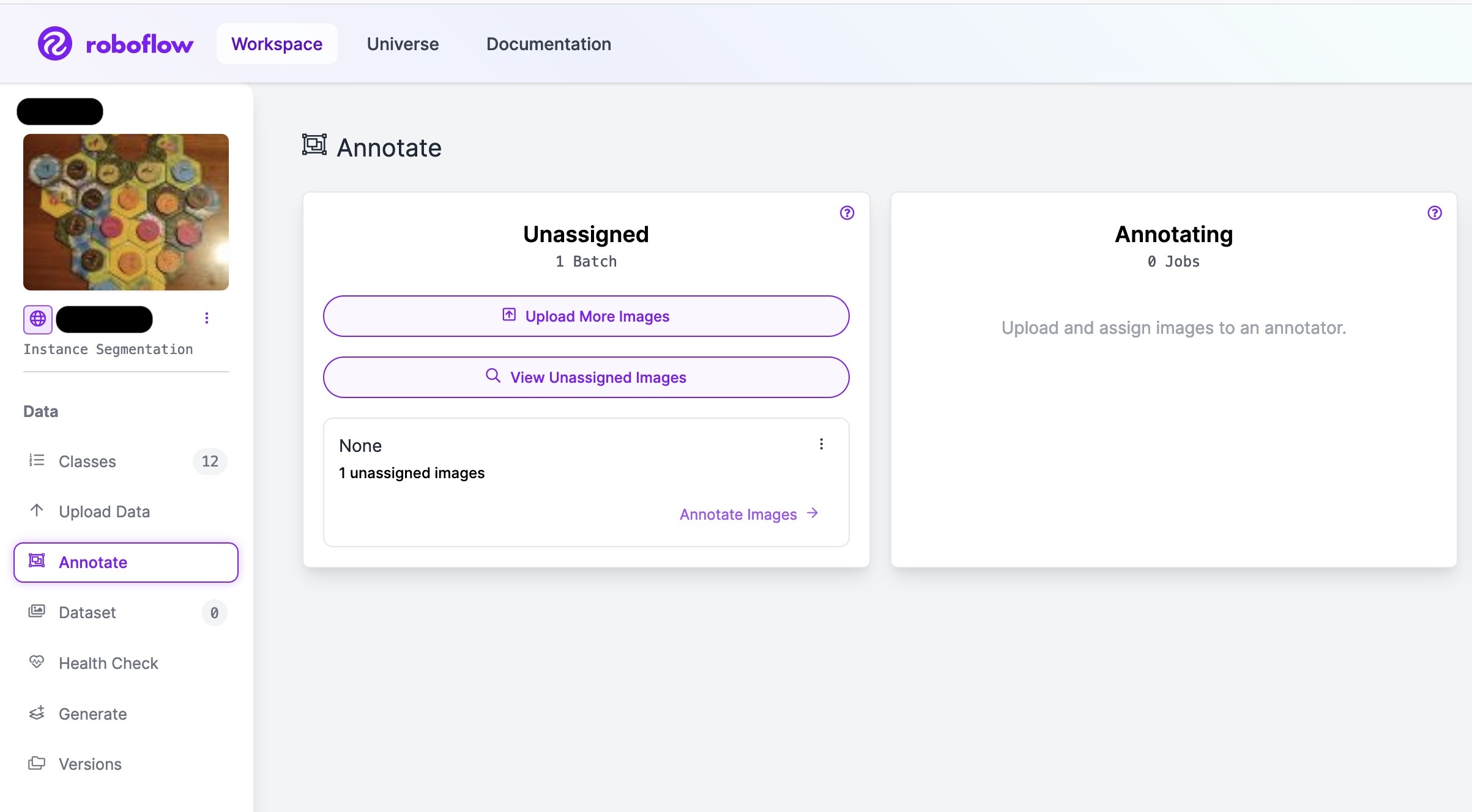
An example of a new unassigned annotation job.
After you start the labeling job and open the image, you will see the pre-annotations. These annotations don’t have a different label, color, or confidence score. They look just like any other annotation. They are still fully editable, so if any of them are wrong, you can click on them and adjust them.
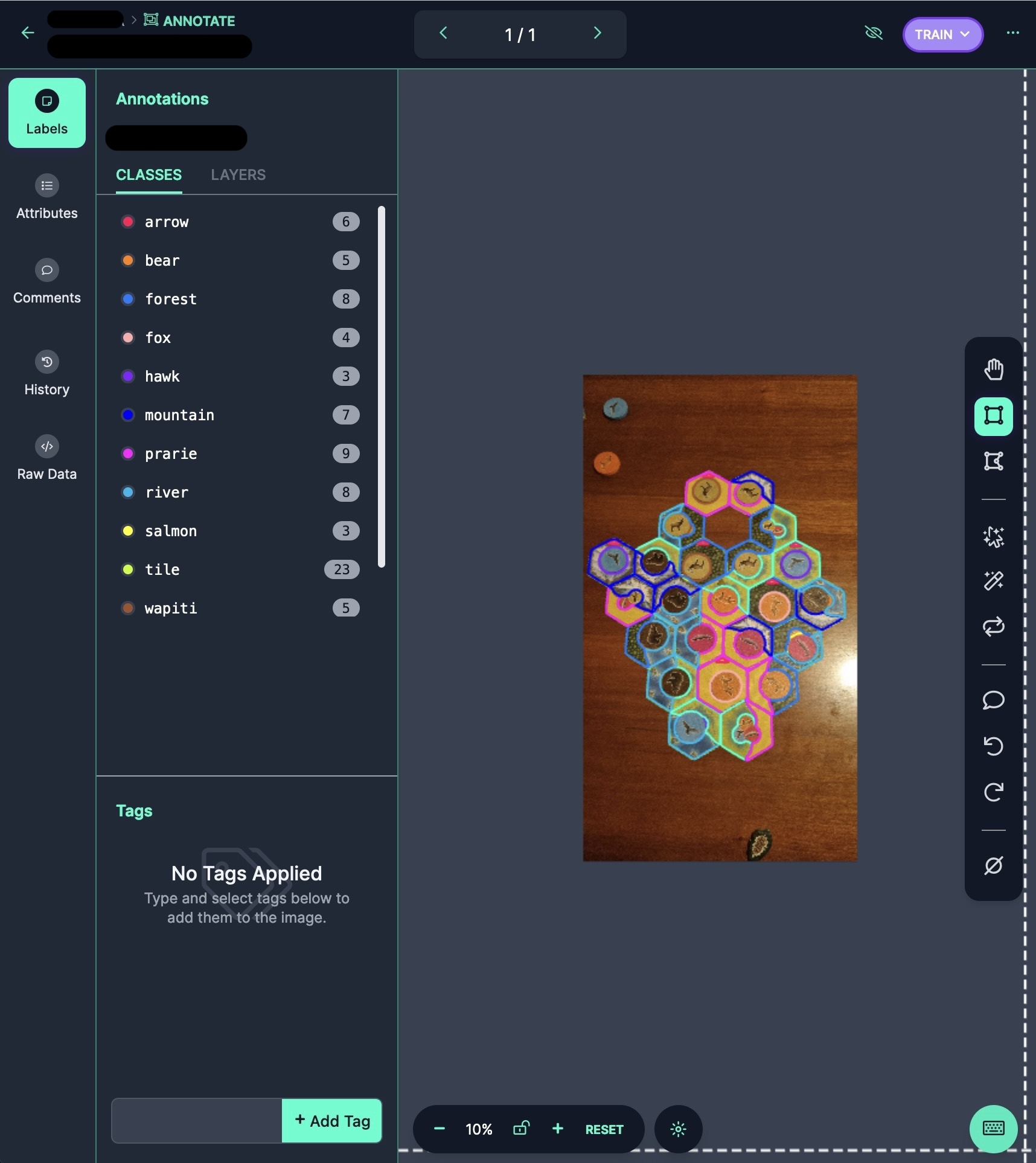
An example of pre-annotations generated by a model. As you can imagine, adjusting these labels is much easier than drawing them from scratch.
Once you are happy, go back to the annotation overview of the labeling job and click on the ‘Add to dataset’ button. Afterward, the pre-annotations will be added to your dataset like any other annotation.
Optional: Down-Sampling of Polygons
When you generate pre-annotations for polygons using a model, you might have too many points in the polygon. When you upload these polygons, it is impossible to adjust them due to the sheer number of points you have to move. To prevent this, you can downsample your polygons before uploading them.
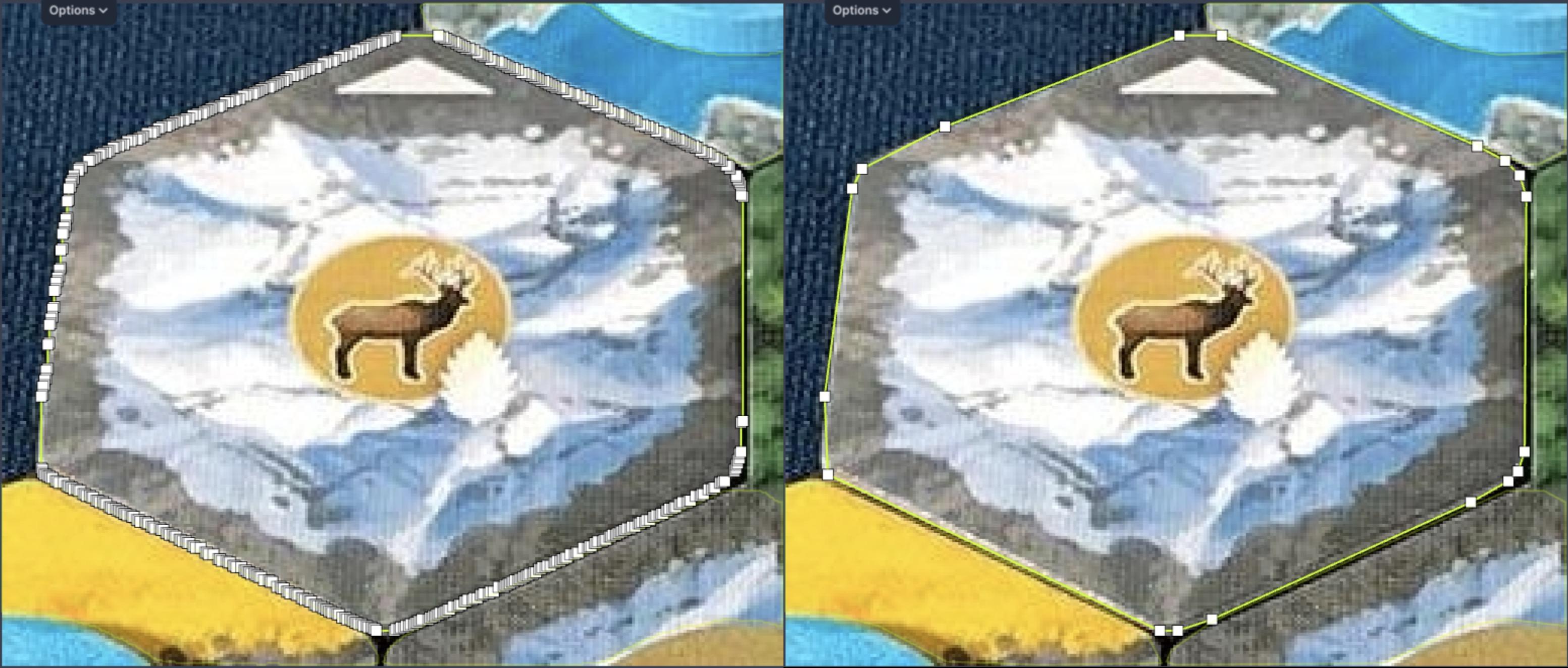
The left polygon is the original predicted polygon, and the right polygon is the down-sampled version. The right polygon is much easier to adjust.
You can down-sample your polygons by removing points that are not essential. This can be done using the Douglas Peucker algorithm. This algorithm finds a polygon that follows a similar path as the original polygon but with fewer points. You can use the following code to down-sample your polygons.
import math


def douglas_peucker(
        points: list[tuple[float, float]],
        epsilon: float,
) -> list[tuple[float, float]]:
    # Find the point with the maximum distance
    dmax = 0.0
    index = 0
    for i in range(1, len(points) - 1):
        d = _distance_from_line(points[i], points[0], points[-1])
        if d > dmax:
            index = i
            dmax = d

    # If max distance is greater than epsilon, recursively simplify
    if dmax >= epsilon:
        # Recursive call
        rec_results1 = douglas_peucker(points[:index + 1], epsilon)
        rec_results2 = douglas_peucker(points[index:], epsilon)

        # Build the result list
        result = rec_results1[:-1] + rec_results2
    else:
        result = [points[0], points[-1]]

    return result


def _distance_from_line(
        point: tuple[float, float],
        line_start: tuple[float, float],
        line_end: tuple[float, float]
) -> float:
    # Calculate the distance of point from the line segment (line_start, line_end)
    if line_start == line_end:
        return math.dist(point, line_start)
    else:
        num = abs((line_end[1] - line_start[1]) * point[0] - (line_end[0] - line_start[0]) * point[1] + line_end[0] *
                  line_start[1] - line_end[1] * line_start[0])
        den = math.sqrt((line_end[1] - line_start[1]) ** 2 + (line_end[0] - line_start[0]) ** 2)
        return num / den
In this algorithm, you can control how much you want to down-sample your polygons by tuning the epsilon parameter.
However, this is a trade-off since more down-sampling means less accurate polygons.
So, use this parameter to find the right balance for your use case.
Wrap Up
To wrap up, using the Roboflow Python SDK to upload annotations and predictions opens up many new possibilities. It has certainly changed how I work with Roboflow. I hope this insight will help you in your future computer vision adventures.