
DIY auto-grad Engine: A Step-by-Step Guide to Calculating Derivatives Automatically
Have you ever marveled at the magic of PyTorch, Jax, and Tensorflow’s auto-grad engines? I know I have! I recently decided to take on the challenge of implementing an auto-grad engine from scratch in Python. It was a fun and humbling experience, and now I want to share my knowledge with you. In this step-by-step guide, I’ll walk you through the process of building your very own DIY auto-grad engine. At the end of this blog, you will understand how these engines automatically calculate derivatives and how you can implement this in Python from scratch. So if you’re ready to dive into the exciting world of auto-grad engines, let’s get started!
Differentiation refresher
Before we start, let’s ensure we’re all on the same math page. If you still know all the differentiation rules from high school, feel free to skip this section. If you need a quick refresher, read on!
Differentiation is a mathematical operation that allows us to find the rate of change of a function with respect to one of its variables. So, if we write $\frac{\partial L}{\partial x}$, we mean the rate of change of $L$ with respect to $x$. If you have a function $L(x)$, you can find the derivative of $L$ with respect to $x$ by applying the differentiation rules, which rule you apply depends on the function $L$. Luckily, you don’t need to remember all the rules because I have created a nice look-up table for you with all the rules you need to know for this post.
| Name | Function | Derivative |
|---|---|---|
| Definition | - | $\frac{\partial L}{\partial L} = 1$ |
| Sum rule | $L = x_1 + x_2$ | $\frac{\partial L}{\partial x_1} = 1$, $\frac{\partial L}{\partial x_2} = 1$ |
| Multiplication rule | $L = x_1 * x_2$ | $\frac{\partial L}{\partial x_1} = x_2$, $\frac{\partial L}{\partial x_2} = x_1$ |
| Chain rule | - | $\frac{\partial L}{\partial x} = \frac{\partial L}{\partial x} \frac{\partial y}{\partial y} = \frac{\partial L}{\partial y} \frac{\partial y}{\partial x}$ |
After you have finished this post, you won’t even need to use this look-up table anymore because your computer will be able to apply all these rules for you automatically! However, before we get there, let’s first review the backpropagation algorithm.
Back propagation
Backpropagation is an algorithm that automatically calculates the functions’ derivatives. It works by constructing a computational graph and then iteratively calculating the gradients of each node based on the chain rule. I can imagine that you’re already thinking: “Well, that sounds a bit vague to me”. So let’s see how this work using a running example. We want to calculate the derivatives of $L$ with respect to every $x_i$:
$$ x_1 = 3 $$ $$ x_2 = 4 $$ $$ x_3 = x_1 * x_2 = 12 $$ $$ x_4 = 5 $$ $$ x_5 = x_3 + x_4 $$ $$ x_6 = 2 $$ $$ L = 34 $$
The first thing we need to do is transform this function into a computational graph. For example, we can view the equation above as the following graph:
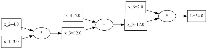
A visualization of the computational graph.
The goal is to find the gradients with respect to $L$ for every node in this computational graph. Calculating the gradients for $x_1$ and $x_2$ looks quite tricky. However, it is a bit easier to find the calculating gradients for $x_5$ and $x_6$ since we can look up their derivation rules in the table above. So, according to the table above, we have:
$$ \frac{\partial L}{\partial L} = 1 $$ $$ \frac{\partial L}{\partial x_5} = x_6 = 2 $$ $$ \frac{\partial L}{\partial x_6} = x_5 = 17 $$ So, let’s update our computational graph with these gradients:
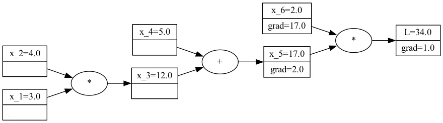
A visualization of the computational graph and the gradients so far.
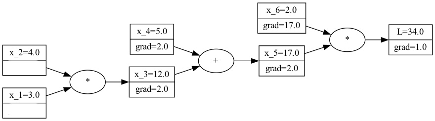
Now, the question is, how do we calculate the gradients for $x_3$ and $x_4$? We know the gradients of $x_5$, which is the parent node of $x_3$ and $x_4$. So, we can use the chain rule and the sum rule to rewrite the gradients for $x_3$ and $x_4$ as follows:
$$ \frac{\partial L}{\partial x_3} = \frac{\partial L}{\partial x_3} \frac{\partial x_5}{\partial x_5} = \frac{\partial L}{\partial x_5} \frac{\partial x_5}{\partial x_3} = 2 *1 = 2 $$
$$ \frac{\partial L}{\partial x_4} = \frac{\partial L}{\partial x_4} \frac{\partial x_5}{\partial x_5} = \frac{\partial L}{\partial x_5} \frac{\partial x_5}{\partial x_4} = 2* 1 = 2 $$
So, by using the chain rule, we change the gradient formula into the local gradient times the gradient of the parent node, which we both know. Let’s continue by filling in these results into our computational graph:
A visualization of the computational graph and the gradients so far.
Thanks to the previous step, the gradient of the parent node of x_1 and x_2 is now known. Therefore, we can again use the chain rule to change the initially complex derivative formulas into the local gradients times the gradient of the parent. $$ \frac{\partial L}{\partial x_1} = \frac{\partial L}{\partial x_1} \frac{\partial x_3}{\partial x_3} = \frac{\partial L}{\partial x_3} \frac{\partial x_5}{\partial x_1} = 2 *3 = 6 $$
$$
\frac{\partial L}{\partial x_2} = \frac{\partial L}{\partial x_2} \frac{\partial x_3}{\partial x_3} = \frac{\partial L}{\partial x_3} \frac{\partial x_5}{\partial x_2} = 2* 4 = 8
$$
This give finally the following computational graph: A visualization of the computational graph with all gradients.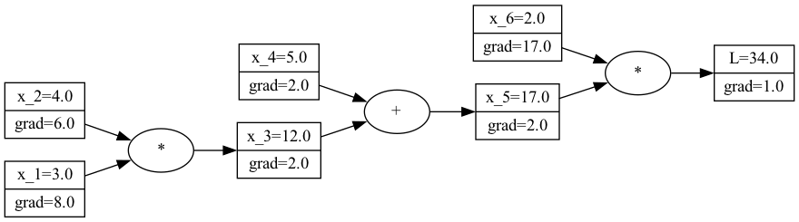
We have now calculated the gradients for every node in the computational graph. With these gradients, we know exactly how changes to any of the $x_i$ will impact the value of $L$. So, let summarize what we have done so far:
- We have constructed a computational graph of the function $L$.
- We set the gradients of the leaf node $L$ to 1.
- We iteratively calculated the gradients of each node in reversed topological order based on the chain rule and the local differentiation rules from the table above.
It is nice that we know how to do this manually, but it is a bit tedious. So, let’s see how we can automate this using an auto-grad engine.
Implementing the Autograd Engine
In this section, we will focus on building a Python data structure that keeps track of the computational graph and local gradients.
This will allow us to perform automatic differentiation, which is the key to implementing an autograd engine.
To keep track of the computational graph and local gradients, we will implement a Value class. This class will have the following attributes:
data: A float representing the current value of the node in the computational graph.children: A set containing the child nodes that contributed to this computation node._backwards: A function that knows how to apply the chain rule to calculate the gradient rule if the parent gradient is known.
This translates to the following __init__ method:
Backwards = Callable[[float], None]

def _noop_grad(_: float) -> None:
    pass

class Value:
    def __init__(
        self,
        data: float,
        children: Optional[set[Value]] = None,
        _backwards: Backwards = _noop_grad,
    ):
        self.data = data
        self.grad = 0.0
        self.children = set() if children is None else children
        self._backwards = _backwards
    ...
Our auto-grad engine needs to be able to construct a computational graph dynamically.
So, for example, if we add two Value objects together, we want to create a new Value object that represents the sum of the two Value objects while keeping track of the underlying computational graph.
We can keep track of this connection by passing the previous Value objects used to construct this node via the children attribute.
We can do this by implementing the __add__ method:
class Value:
   ...
   def __add__(self, other: Value) -> Value:
       def _backward(grad_parent: float) -> None:
           self.grad += grad_parent
           other.grad += grad_parent

       return Value(
           self.data + other.data,
           children={self, other},
           _backwards=_backward,
       )
   ...
This implementation of the __add__ method does the following:
- It calculates the data value for the new
Valueobject by adding the data values of the twoValueobjects. - Here we define how to calculate the gradient of
selfandotherin the_backwardfunction. This function takes as input the gradient of the parent node and calculates the gradient of the child nodes. This is the chain rule in action, exactly as we did manually in the previous section. - It keeps track of the
childrenof the newValueobject. This is the computational graph connection.
Now, we can do a single gradient calculation as follows:
x_1 = Value(1)
x_2 = Value(2)
l = x_1 + x_2

l._backwards(1)
assert x_1.grad == 1
assert x_2.grad == 1
At this point our _backwards function only works for a computational graph that is a single layer deep.
So, let’s extend our auto-grad engine to support more complex computational graphs.
To do this, we need to implement the backward method.
This will set the gradient of the root node to 1 and then recursively call the _backwards method on all the child nodes in reversed topological order.
You might ask yourself why we need to do this in reversed topological order?
The reason for this is that we can only use the _backwards method if we know the gradient of the parent node.
If we iterate over the node in reversed topological order, the gradient of the parent node is always known when we call the _backwards method.
So, let’s implement the backward method:
class Value:
    ...

    def backward(self) -> None:
        self.grad = 1

        for v in find_reversed_topological_order(self):
            v._backwards(v.grad)

    ...

def find_reversed_topological_order(root: Value) -> list[Value]:
    visited = set()
    topological_order = []

    def _depth_first_search(node: Value):
        if node not in visited:
            visited.add(node)

            for child in node.children:
                _depth_first_search(child)

            topological_order.append(node)

    _depth_first_search(root)

    return list(reversed(topological_order))
In this implementation, we use a depth first search to find the reversed topological order.
Now, with the backwards method implemented, we can do a gradient calculation on deeper and more complex computational graphs as follows:
x_1 = Value(1)
x_2 = Value(2)
x_3 = Value(3)
x_4 = Value(4)
l = x_1 + x_2 + x_3 + x_4

l.backwards()
assert l.grad == 1
assert x_1.grad == 1
assert x_2.grad == 1
assert x_3.grad == 1
assert x_4.grad == 1
That is great! Our auto-grad engine now works for arbitrary deep computational graphs. Sadly, it only works with additions. So, let’s extend our auto-grad engine to support more operations. Let’s start with multiplication:
class Value:
    ...
    def __mul__(self, other: Value) -> Value:
        def _backward(grad_parent: float) -> None:
            self.grad += other.data * grad_parent
            other.grad += self.data * grad_parent

        return Value(
            self.data * other.data,
            children={self, other},
            _backwards=_backward,
        )

    ...
Notice that this looks very similar to the __add__ method.
The only differance is that we use the local differentiation rule for multiplication in the _backward function.
Everything else is the same.
Now, with the multiplication we can verify that our auto-grad engine can solve the computational graph we solved manually in the previous section:
x_1 = Value(3)
x_2 = Value(4)
x_3 = x_1 * x_2
x_4 = Value(5)
x_5 = x_4 + x_3
x_6 = Value(2)
l = x_5 * x_6

l.backwards()

print(f"date={x_1.date} grad={x_1.grad}") # date=3 grad=8
print(f"date={x_2.date} grad={x_2.grad}") # date=4 grad=6
print(f"date={x_3.date} grad={x_3.grad}") # date=12 grad=2
print(f"date={x_4.date} grad={x_4.grad}") # date=5 grad=2
print(f"date={x_5.date} grad={x_5.grad}") # date=17 grad=2
print(f"date={x_6.date} grad={x_6.grad}") # date=2 grad=17
print(f"date={l.date} grad={l.grad}")     # date=34 grad=1
Our auto-grad engine now supports addition and multiplication. Of course there are many more operations that we can support, like subtraction, division, exponentiation, etc. However, I want to leave those as an exercise for the reader. To make this exercise a bit easier, I have created a GitHub repository with the code we have written so far. It also contains a test suite that you can use to verify your implementation and solutions if you get stuck.
Conclusion
In this blog post, we delved into the backpropagation algorithm and how it can be used to calculate gradients in a computational graph. We then automated this process by implementing a mini auto-grad engine. During this process, we learned that auto-grad engines are not magic but rather smart data structures that apply the chain rule automatically. Despite this, they are handy for calculating gradients with ease.
I hope this tutorial was helpful and that you were able to follow along and implement your own auto-grad engine.